Deep Learning Modellanpassungen

Bias / Varianz

Trade off von Bias und Varianz

„In statistics and machine learning, the bias–variance tradeoff is the property of a model that the variance of the parameter estimates across samples can be reduced by increasing the bias in the estimated parameters. The bias–variance dilemma or bias–variance problem is the conflict in trying to simultaneously minimize these two sources of error that prevent supervised learning algorithms from generalizing beyond their training set:

• The bias error is an error from erroneous assumptions in the learning algorithm. High bias can cause an algorithm to miss the relevant relations between features and target outputs (underfitting).

• The variance is an error from sensitivity to small fluctuations in the training set. High variance can cause an algorithm to model the random noise in the training data, rather than the intended outputs (overfitting).

This trade-off is universal: It has been shown that a model that is asymptotically unbiased must have unbounded variance. The bias–variance decomposition is a way of analyzing a learning algorithm’s expected generalization error with respect to a particular problem as a sum of three terms, the bias, variance, and a quantity called the irreducible error, resulting from noise in the problem itself.“ [ Bias Variance TradeOff ]

Beispiel: Quelle: Andrew Ng, Coursera, Improving Deep Learning

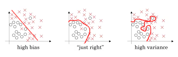
Abb. 6: Bias Varianz (Abb. 6)

• links: Beispiel für ein hohes Bias. Hohe Fehlerrate bei den vorhergesagten Werten (Underfitting)

• rechts: Beispiel für eine hohe Varianz. Das Modell auf Basis der Trainingsdaten ist zu spezifisch, so dass das Modell schlecht an den realen Daten skalieren kann. (Overfitting)

• Mitte: optimaler Beziehung zw. Fehlern auf der einen Seite und Komplexität des Modells auf der anderen Seite.

Beispiel für die Beurteilung ^*):

	Fehlerrate
Test-Set	1%	15%	15%	0.5%
Development-Set	11%	16%	30%	1%
Beurteilung	overfitting, hohe Varianz	underfitting, High Bias	high bias, high variance	low bias, low variance

^*): Alle Werte werden in Relation zu einer Fehlerrate beim Menschen beurteilt, in diesem Fall liegt dieser bei annnährend 0% (auch Bayes Fehler genannt)

Zurück zu Deep Learning Modellanpassungen

Basisprozess im Machinelearning

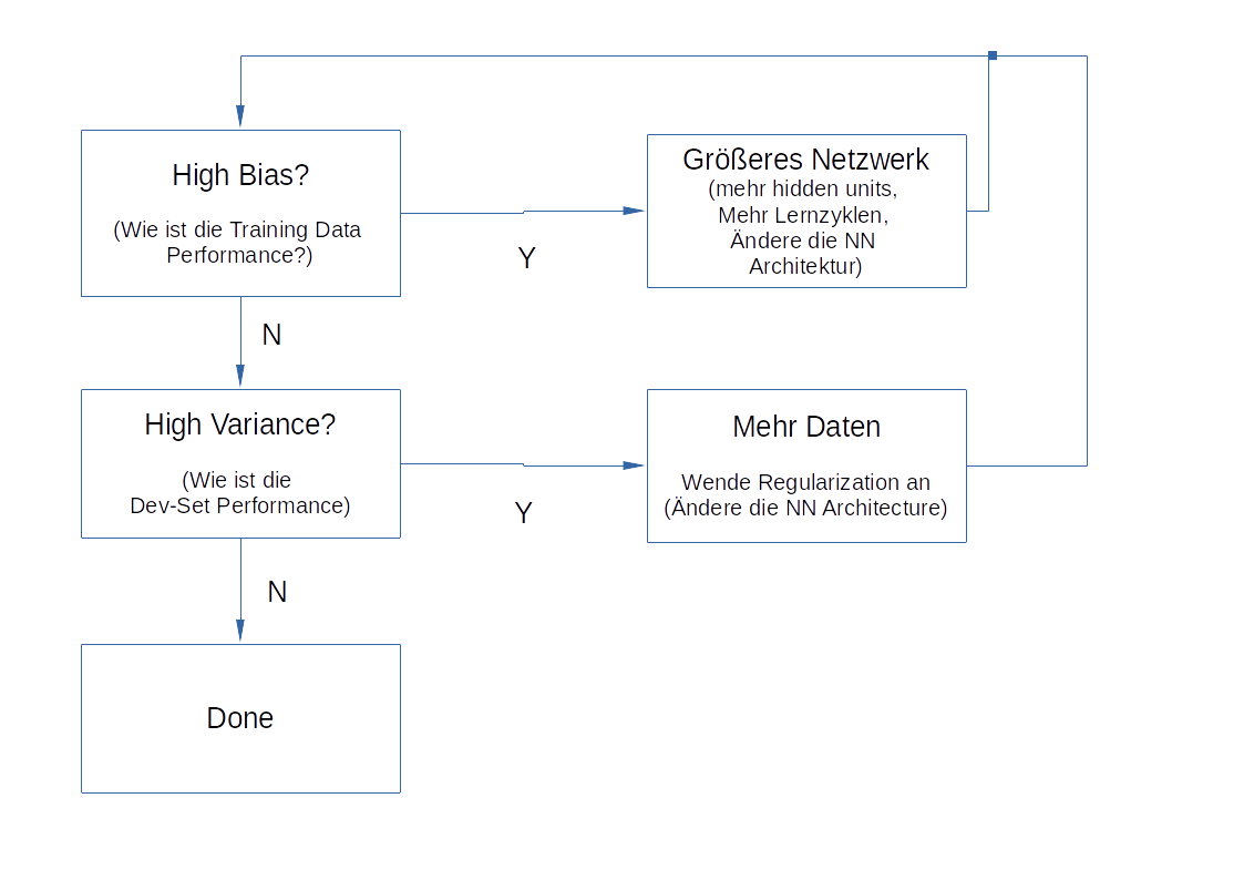
Abb. 7: Basis ML Prozess (Abb. 7)

Zurück zu Deep Learning Modellanpassungen

Regularization

Über „Regularization“ kann Einfluss auf Bias und Varianz genommen werden.

Regularization in Logistic Regression

Ziel ist die Minimierung der Funktion J(w,b)

\(min(w,b) \rightarrow J(w,b)\)

Man addiert die Regularization zur Funktion. Unterschieden wird zwischen L1 und L2 Regularization, L2 wird typischerweise verwendet.

\(L_{2}\) Regularization = \(\|w\|^{2}_{2}=\sum^{N_x}_{j=1}w^{2}_{j}=w^{T}w\)

Daraus folgt für die zu minimierende Funktion: \(J(w,b)=\frac{1}{m} \sum^{m}_{i=1}L(\hat y^{(i)}, y^{(i)})+ \frac{\lambda}{2m}\|w\|^{2}_{2}\)

Der Vollständigkeit halber: \(L_{1}\) Regularization = \(\frac{\lambda}{2m}\sum^{N_x}_{i=1}|w|=\frac{\lambda}{2m}\|w\|_{1}\)

w ist ein Vektor mit vielen Nullen, damit kann das Modell komprimiert werden (dies ist in der Praxis eher nachrangig)

\(\lambda=\) ist ein Regularization Parameter und kann ebenfalls angepasst werden.

Regularization in Neuronalen Netzwerken

Analog dem Vorgehen aus der Regularization logistic regression ergibt sich für ein NN:

\(J(w^{[1]},b^{[1]},...,w^{[i]},b^{[i]}) = \frac{1}{m} \sum^{m}_{i=1}L(\hat y^{(i)}, y^{(i)})+ \frac{\lambda}{2m} \sum^{L}_{l=1}\|w^{[l]}\|^{2}_{F}\)

wobei \(\|w^{[l]}\|^{2}=\sum^{n^{[l-1]}}_{i=1} \sum^{n^{[l]}}_{j=1}(w^{[l]}_{ij})^{2}\)

\(w: (n^{[l]},n^{[l-1]})\) ist die Matrix mit den Dimensionen der Hidden Layer n und n-1.

Man spricht hier nicht von der L2 Regularization sondern von der „Frobenius norm“. Dies wird in der obigen Gleichung durch ein runtergestelltes F dargestellt.

Implementierung von Gradient Descent in dieses Modell:

(1): \(dw^{[l]} = (from \: backpropagation)+\frac{\lambda}{m}w^{[l]}\)

Für \(w^{l}\) gilt (2): \(w^{[l]}=w{[l]}-\alpha \: dw^{[l]}\)

Setzt man (1) in (2) ergibt sich:

\(w^{[l]} = w^{[l]}-\alpha[(from \: backpropagation)+\frac{\lambda}{m}w^{[l]}]\)

\(w^{[l]} = w^{[l]}-\frac{\alpha \lambda}{m}w^{[l]}-\alpha(from \: backpropagation)\)

Dies kann man vereinfachen, zieht man auf der rechten Seite die Matrix w vor die Klammer, dann ergibt sich daraus, dass von der w-Matrix jeweils der Wert \((1-\frac{\alpha \lambda}{m})\) abgezogen wird.

Dropout

Dropout ist eine andere Form der Regularization. Beim Dropout geht man durch jeden Layer und „löscht“ Knoten auf Basis von Wahrscheinlichkeiten. Beispielsweise wird je Layer einer Wahrscheinlichkeit von 0.5 ein Knoten je Layer eleminiert. Man löscht dann die Verbindung zu dem Knoten. Das so verkleinerte NN ist weniger Komplex und kann schneller berechnet werden.